-
Notifications
You must be signed in to change notification settings - Fork 13
Tutorial: Using an Extension
This tutorial runs through the methods used to generate analyses and figures used in Hinman et al 2016 http://www.cell.com/neuron/fulltext/S0896-6273(16)30305-1. Please note that the tutorial below requires the corresponding CMBHOME extension, which can be cloned from https://github.com/hasselmonians/SpeedLFP.
We assume a CMBHOME.Session object is loaded in the workspace as root, and has root.cel and root.active_lfp set.
The firing rate of the neuron as a function of running speed was created using three different methods.
This is the "traditional" method of determining the speed modulation of a neuron, and is done by taking the speed at each spike time, binning into 1cm/s speed bins, and dividing the number of spikes by the total amount of time spent in that speed bin. This is implemented as SpeedMod.
figure();
[f_cell, vel_dim] = SpeedMod.BinnedVelocityFR(root);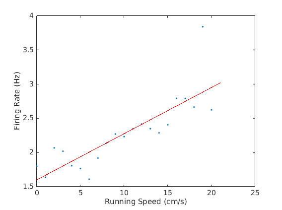
We now see the average firing rate in each of the velocity bins. If the extension weren't available then you could rewrite the binned velocity:
function [f_cell, vel_dim] = BinnedVelocityFR(root, vel_dim, plotit)
% Calculates the rate of firing for cell cel, for bins of running speed.
%
% If vel_dim is specified, bin edges of running speed are vel_dim
% If vel_dim is not specified, bin edges of running speed are [0 max_vel]
% in increments of 1 cm sec^-1.
%
% Remember that root.spatial_scale sets cm/pixel.
%
% If multiple epochs are set in root.epoch, then all data from each epoch
% are concatinated and analysed as continuous
%
% root.epoch needs to be 1x2 vector
%
%[F, V] = root.VelocityRate(cel, vel_dim)

if ~exist('vel_dim', 'var')
    vel_dim = 0:root.spatial_scale^-1:prctile(CMBHOME.Utils.ContinuizeEpochs(root.vel),95);
end
if ~exist('plotit','var')
    plotit=1;
end

if isempty(root.b_vel), disp('Warning, no user specified velocity assigned. The simple derivative thus used may not be optimal for this analysis'); end

import CMBHOME.Utils.*
root = MergeEpochs(root);
[vel, spk_vel] = ContinuizeEpochs(root.vel, root.cel_vel); % get running speed at spikes
tao_v = histc(vel, vel_dim) .* root.fs_video^-1; % time spent in each bin of running speed
spikes_v = histc(spk_vel, vel_dim);% spikes in each bin of running speed
f_cell = spikes_v ./ tao_v;
vel_dim = vel_dim(:);

%% Fit Params
[y_m, R, P, b, y_int] = CMBHOME.Utils.LinearRegression(vel_dim,f_cell);

%%
if plotit==1
     plot(vel_dim*root.spatial_scale, f_cell,'.');
     hold on
     plot(vel_dim*root.spatial_scale,vel_dim*b+y_int,'r')
     xlabel('Running Speed (cm/s)');
     ylabel('Firing Rate (Hz)')
endThis method is based on the Kropff et al 2015 paper (http://www.nature.com/nature/journal/v523/n7561/full/nature14622.html), where the lab calculated an "instantaneous firing rate" by smoothing delta functions at the spike times. This is implemented in SpeedMod.
figure();
[R, root, frFilt] = SpeedMod.InstFR(root, 1);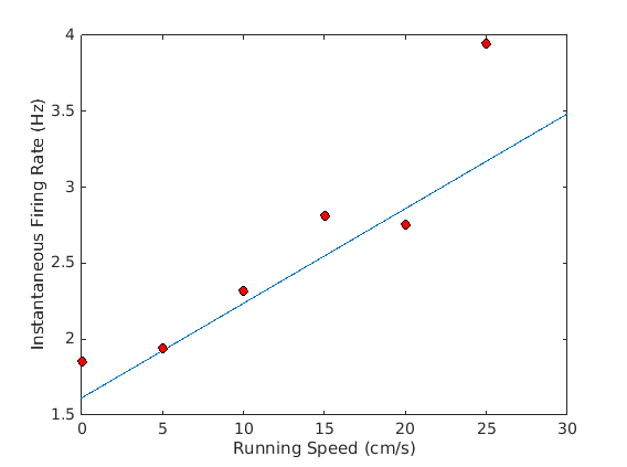
Again, walking through the code in the extension:
function [R, root, frFilt] = InstFR(root, ifPlot)
    % Speed Cell regression as in Kropff 2015
    % [R, root, frFilt] = SpeedMod.InstFR(root, ifPlot)
    %
    % http://www.nature.com/nature/journal/v523/n7561/full/nature14622.html
    if ~exist('ifPlot','var')
        ifPlot = 0;
    end

    %% Instantaneous firing rate
    root.epoch = [-inf inf];
    fr = zeros(size(root.x));
    temp = root.spike(root.cel(1), root.cel(2)).i;
    tt = unique(temp);
    for i = 1:length(tt)
        fr(tt(i)) = sum(temp == tt(i));
    end

    sigma = 33/(1000/(root.fs_video));
    ssize = floor(10*sigma);
    x = linspace(-ssize / 2, ssize / 2, ssize);
    gaussFilter = exp(-x .^ 2 / (2 * sigma ^ 2));
    gaussFilter = gaussFilter / sum (gaussFilter); % normalize
    frFilt = conv (fr, gaussFilter, 'same');
    frFilt = frFilt * root.fs_video;
    root.b_myvar = frFilt;

    %%
    R = corr(root.vel, root.myvar);

    if ifPlot == 1
        vd = (0:5:30)/root.spatial_scale;
        sp = [0, prctile(root.vel, 95)];
        [y_m, R, P, b, y_int] = CMBHOME.Utils.LinearRegression(root.vel, root.myvar);
        ym = sp * b + y_int;
        plot([0 30], [0 30]*(b/root.spatial_scale)+y_int)
        hold on
        [~,wb] = histc(root.vel, vd);
        for k = 1:max(wb)
            mv(k) = mean(root.myvar(wb==k));
        end
        plot(vd(1:end-1)*root.spatial_scale, mv,'ko','MarkerFaceColor','r')
        xlabel('Running Speed (cm/s)');
        ylabel('Instantaneous Firing Rate (Hz)')
    end

endfigure();
[ stats ] = SpeedMod.PoissonFR(root, 1);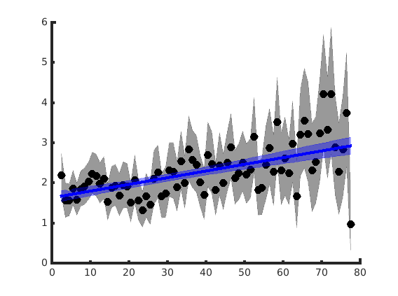
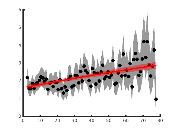
A rather good example usage of this lives on its home (github.com/jrclimer.mle_rhythmicity), so we ignore it here, especially as the internals do not make use of the CMBHOME Toolbox.
Finally, we analyzed spiking phase (relative to theta band of the local field potential) as a function of running speed. Because the @LFP structure aligns to the behavioral data (@Session) this is easy to implement:
vel_dim = (0:5:50);
[~,wb] = histc(CMBHOME.Utils.ContinuizeEpochs(root.vel), vel_dim);
root.epoch = [-inf inf];
oe = root.epoch;
prefered=NaN(length(vel_dim)-1,1); erv = prefered; prefered_mrl=prefered;

for i = 1:(length(vel_dim)-1)
    root.epoch = oe;
    root = root.RunningEpochs(vel_dim(i), vel_dim(i+1), 1);
    tp = CMBHOME.Utils.ContinuizeEpochs(root.cel_thetaphase);
    prefered(i) = wrapToPi(CMBHOME.Utils.circ.circ_mean(tp));
    erv(i) = CMBHOME.Utils.circ.circ_std(tp);
    prefered_mrl(i) = CMBHOME.Utils.circ.circ_r(tp);
end

% linear fit
vdm = mean([vel_dim' [vel_dim(2:end)';NaN]],2); vdm=vdm(1:end-1);
[x,phi,a,phi_knot,rho_c,p] = CMBHOME.Utils.corrC2L(vdm,prefered);


% plotting
figure();
hold on
plot(root.cel_vel{1}*root.spatial_scale,root.cel_thetaphase{1},'b.')
plot(root.cel_vel{1}*root.spatial_scale,root.cel_thetaphase{1}+2*pi,'b.')
plot(root.cel_vel{1}*root.spatial_scale,root.cel_thetaphase{1}-2*pi,'b.')
errorbar(vdm,prefered,erv,'r','LineWidth',1);
axis([0 max(vel_dim) 0 2*pi])
xlabel('Velocity (cm/s)')
ylabel('Thetaphase @ cellSpike')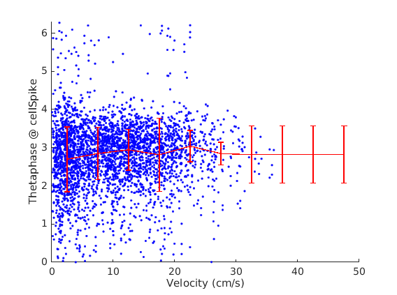
As a sidenote and general tutorial, if you were interested in an LFP property that's not inherently part of the toolbox (ie; some other frequency band), you can still have the toolbox do the dirty alignment work:
% Create your property, in this case just a random signal of same sampling frequency as LFP
myvar = rand(size(root.b_lfp(root.active_lfp).ts);
% Assign as lfp.myvar:
root.b_lfp(root.active_lfp).b_mybar = myvar;

% Use spike.i
cel_inds = root.spike(root.cel(1),root.cel(2)).i_lfp{1};
cel_lfpmyvar = root.b_lfp.myvar(cel_inds);
plot(root.cel_vel{1}, cel_lfpmyvar{1});
Copyright (c) 2016, Trustees of Boston University, All Rights Reserved