Displacement Integration for Dynamic Analysis

This Python script allows for the integration of an accelerogram to obtain the temporal history of displacement.

Table of contents

• Description
• Dependencies
• Usage
• Examples
• Remarks

Description

In dynamic structural analyses, a very dense sampling of the accelerogram is typically used, in the order of hundredths of a second. When performing a dynamic analysis using a temporal history of displacements, the sampling interval must be denser. This script automatically generates a temporal history of displacements with a user defned sampling interval. It is also possible to specify initial boundary conditions in terms of displacement and velocity.

This script allows performing integration using two methods:

• Wilson algorithm See the CSI Wiki
• Fourth-order Runge-Kutta algorithm See the Wiki page

Additionally, it performs a linear baseline correction of the velocity and displacement output.

Temporal displacement histories are used for various purposes in structural engineering, such as seismic analyses that consider the effect of seismic motion propagation, typically in bridges. Other examples include analyses of moving components within the structure.

Here are two practical examples:

Example 1: Integrating a seismic accelerogram sampled at 1/100 seconds into displacement at 1/1000 seconds.

Example 2: Integrating an accelerogram derived from a dynamic analysis of a moored ship subjected to wind and waves, performed using Orcaflex. The displacement history derived from Orcaflex is compared to that derived from double integration executed with the script.

Dependencies

To use this script, it is necessary to install the following libraries that are used:

• numpy
• scipy
• matplotlib

To install them, you can use pip:

    pip install numpy
    pip install scipy
    pip install matplotlib

Usage

The script consists of a main module named integrate_module.py containing functions for performing double integration. The functions included are:

• integrate_wilson: Integrates an accelerogram using the Wilson method to determine the history of velocity and displacements based on boundary conditions.
• integrate_rk4: Integrates an accelerogram using the fourth-order Runge-Kutta method to determine the history of velocity and displacements based on boundary conditions.
• baseline: Performs a baseline function that linearly corrects the passed function while preserving the initial conditions.

To use these functions, it's necessary to import them into the script performing the computation, for example:

from integrate_module import integrate_wilson, baseline

Based on the chosen integration algorithm, it will be used in the execution; both will be utilized in the two provided examples.

The input file containing the accelerogram must be formatted as follows:

• It must not contain headers.
• The first column should contain the time values.
• The second column should contain the accelerations.
• The separator should be a semicolon.

The output will have the same unit of measurement as the input. Therefore, if the acceleration is in m/s^2, the displacement will be in meters.

Two examples have been developed to test the script, which also serve as a reference for how to use it.

Examples

Example 1

The first example involves the integration of a seismic accelerogram spectrum-compatible generated using the Simqke algorithm developed at Berkeley. The accelerogram has a sampling interval of 1/100 of a second and a total duration of 30 seconds.

Subsequently, the integration is performed using the Wilson algorithm with an integration step of 1/1000 seconds. The result is compared with an integration executed through the finite element analysis software SAP2000 from CSI.

This is a classic example of creating a temporal history of displacements to perform a finite element dynamic analysis.

This example is set up in the script Example1.py.

At the beginning of the file Exemple1.py, the necessary functions are imported:

from integrate_module import integrate_wilson, baseline

And the parameters for integration are set:

Define the file path containing the accelerogram
file_path = 'seismic_accelerogram.txt'

Set the initial conditions:
y0 = 0  # Displacement
v0 = 0  # Velocity

Set the desired time step for the output
dt = 0.001

The output of the script is shown in the following figure, the numerical values of the temporal displacement history are saved in the CSV file named displacement_record.csv.

The displacement history is then compared with the one determined using the finite element software SAP2000. The integration performed through SAP2000 has the same integration step of 1/1000, and the integration algorithm used is the Newmark method. The result of the comparison is shown in the following figure.

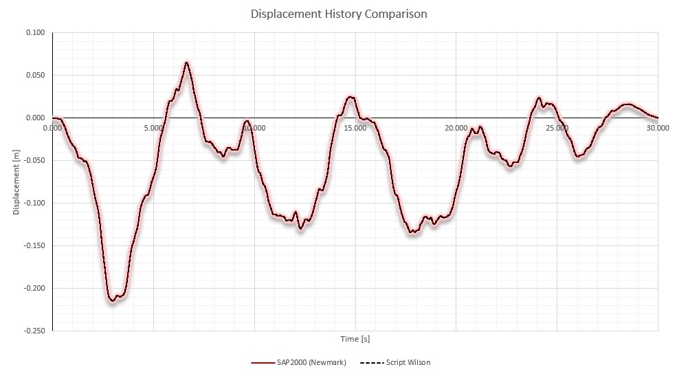
To assess the discrepancy between the two temporal displacement histories, the root-mean-square error (RMSE) was calculated, resulting in 0.014%, indicating an excellent agreement between the two solutions.

Example 2

This second example demonstrates the integration of an accelerogram derived from a dynamic analysis of a moored ship subjected to wind and waves, performed using Orcaflex.

It considers an acceleration history due to the sway of the ship. For this simulation, both the acceleration and displacement histories are available, sampled at 1/100 seconds and lasting 340 seconds.

The displacement history obtained from Orcaflex is compared to that derived from double integration executed with the script.

The temporal history presents an initial condition of acceleration, velocity, and displacement that are not equal to zero. The accelerogram is passed to the script as is, and initial conditions of velocity and displacement are set. The time step for the displacement history remains the same as that of the accelerogram, allowing for a more precise comparison with the displacement history derived from the Orcaflex analysis. For this example, the Runge-Kutta integration algorithm is used.

This example is set up in the script Example2.py.

At the beginning of the file Exemple2.py, the necessary functions are imported:

from integrate_module import integrate_rk4, baseline

And the parameters for integration are set:

Define the file path containing the accelerogram
file_path = 'vessel_accelerogram.txt'

Set the initial conditions:
y0 = 0.021491332862909 # Displacement
v0 = 0.0176782812923192 # Velocity

Set the desired time step for the output
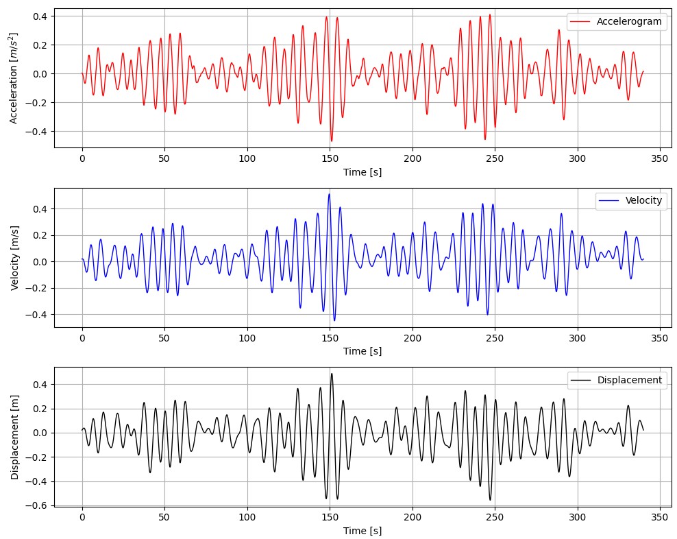
dt = 0.01

The output of the script is shown in the following figure, the numerical values of the temporal displacement history are saved in the CSV file named displacement_record.csv.

The temporal history of displacements has been compared with that derived from the dynamic analysis conducted using Orcaflex. The result of the comparison is shown in the following figure.

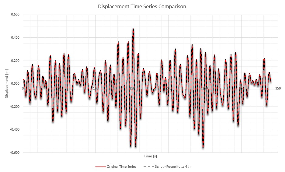
To assess the discrepancy between the two temporal displacement histories, the root-mean-square error (RMSE) was calculated, resulting in 0.227%, indicating an excellent agreement between the two solutions.

Remarks

I am posting this script on GitHub as a personal backup and for anyone who intends to use it. I want to clarify that I am not responsible in any way for the usage or the accuracy of the obtained results. The conditions of use vary widely, and for more complex analyses, different integration algorithms, tools to correct the input accelerogram, or filters for the output displacement might be necessary.