How it Works
Here are some more details about how RenderToolbox works.
Let's start with an example. We'll take a 3D dragon scene, apply some conditions and mappings to change the color of the dragon, do some rendering, then make a nice montage.
We'll start with a dragon model which was produced at Stanford University and made available at MrBlueSummers.com.
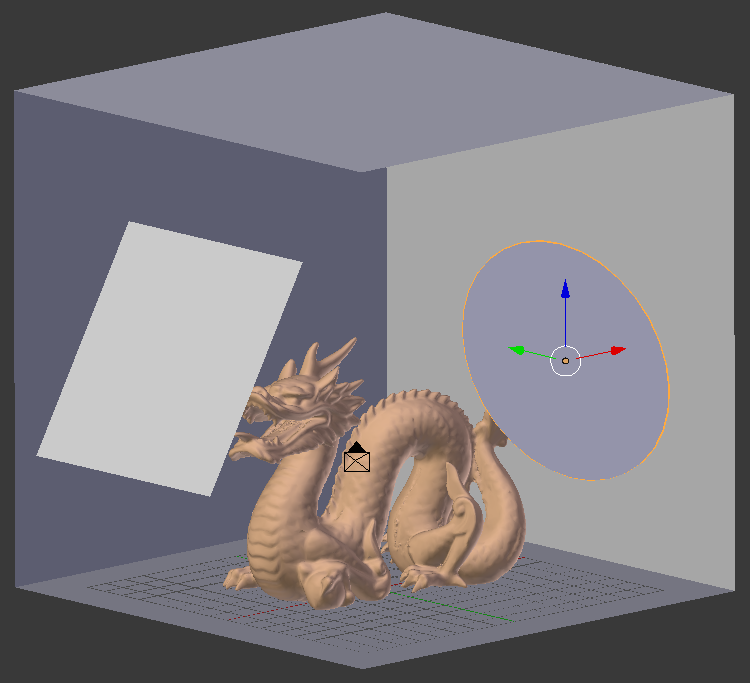
We imported this model into Blender to add a box for the dragon to sit in, some meshes to act as area lights, and a camera. Here's a screen shot from Blender:
RenderToolbox can read the .blend files saved by Blender. Under the hood, it uses a library called Assimp to load the scene into memory, then uses a wrapper called mexximp to convert the scene into a Matlab struct.
Assimp and mexximp are handy tools that you might wish to use with or without RenderToolbox.
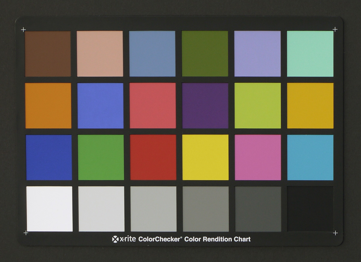
For this example, we would like to render the dragon scene many times, each time with a different surface reflectance for the dragon. We will use the 24 ColorChecker reflectances that are included with RenderToolbox. Here's a photo of a real-life ColorChecker chart:
We can add ColorChecker reflectances to our scene by way of a Conditions File. This is a text file with columns of variables and rows of values. In this example, we have a column for the image name, and a column for the name of a ColorChecker spectrum file. We have a row for each square on the ColorChecker chart:
imageName         dragonColor
macbethDragon-1	  mccBabel-1.spd
macbethDragon-2	  mccBabel-2.spd
macbethDragon-3	  mccBabel-3.spd
macbethDragon-4	  mccBabel-4.spd
macbethDragon-5   mccBabel-5.spd
...               ...
RenderToolbox will create a variant of the original dragon scene, one for each row in the conditions file. Note the name of the second column, dragonColor. This is a variable name that we will use below.
The conditions file is just a text file with values organized into rows and columns. To connect these values to the scene, we need to do some kind of mapping from the conditions file to elements of the 3D scene. For this we use a Mappings File.
RenderToolbox mappings files are JSON documents that identify elements of the 3D scene and assign values to them. Here's an excerpt for the dragon scene:
  {
    "name": "DragonMaterial",
    "broadType": "materials",
    "operation": "update",
    "specificType": "matte",
    "properties": {
      "name": "diffuseReflectance",
      "valueType": "spectrum",
      "value": "(dragonColor)"
    }
  }
This JSON object identifies a material with the name DragonMaterial. This was a name we typed into Blender when creating the scene. It specifies that we want to update the material to have the type matte -- that is, we want the Dragon to have Lambertian reflectance.
It further specifies that we want to update a property of the material named diffuseReflectance. This property takes a spectrum value. The value we are assigning comes from a variable named dragonColor, which corresponds to a column in the conditions file, above.
In short: this JSON object maps dragonColor values from the conditions file to the diffuseReflectance property of the dragon's material.
As RenderToolbox processes the dragon scene, conditions file, and mappings file, it will produce scene files suitable for specific renderers. In this example, PBRT and Mitsuba.
Under the hood, RenderToolbox uses object-oriented models of renderer scene formats. These make it possible to create and modify the native scene representations during batch processing, before dumping out actual renderer scene files.
The object-oriented models are called mPbrt and mMitsuba. These are handy tools that you might wish to use with or without RenderToolbox.
RenderToolbox takes care of invoking each renderer to perform the rendering, and reading the multi-spectral image files from each renderer back into Matlab.
The multi-spectral image files produced by renderers contain lots of information. But they're hard to view because they're not RGB. RenderToolbox provides a number of image processing utilities for converting multi-spectral images to RGB for viewing, or to other "sensor images" based on arbitrary color matching functions.
These utilities are based on Psychtoolbox-3, which is a handy tool you might wish to use with or without RenderToolbox.
For this example we had 24 multi-spectral data files, one for each square on the ColorChecker chart. We converted each one to RGB for viewing, and assembled them all into a montage that resembles the original chart:

Making a montage like this is only one possibility. Once you have the multi-spectral images in Matlab, you can process them and analyze them however want.
The dragon scene gives one specific example of how RenderToolbox works. Here is a flow chart outlining the general RenderToolbox workflow:
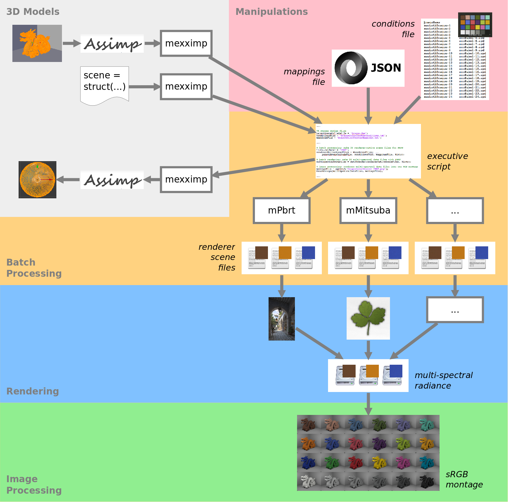
In the gray box in the top-left, we have 3D models. Assimp is able to import many 3D model formats and mexximp is able to bring these into Matlab.
It's also possible to use mexximp to create scenes from scratch, entirely in Matlab.
Finally, mexximp is able to take scene data in Matlab and push it out to Assimp. In turn, Assimp is able to export scene data to several 3D model formats.
In the red box in the top-right, we have scene manipulations. These are specified as variables and values in a Conditions File. The values are mapped to the 3D scene by way of a Mappings File.
In the orange box in the upper-middle, we have batch processing. This begins with an executive script that pulls together the 3D scene, conditions file, and mappings file, and invokes RenderToolbox functions.
In turn, RenderToolbox uses tools like mPbrt and mMitusba to generate renderer-native scene files. It may generate many such files, one for each row of the conditions file.
In the blue box in the lower-middle, we have Rendering. RenderToolbox takes care of invoking renderers like PBRT and Mitsuba with the generated scene files, and reading multi-spectral outputs from the renderers back into Matlab.
RenderToolbox was written and tested with PBRT and Mitsuba in mind. We make pre-built renderers available as Docker images.
It would be possible to support additional as well, by extending the Renderer and Converter classes.
Finally, RenderToolbox provides several utilities for processing and analyzing the multi-spectral images produced by the renderers.
This may be where you write most of your own code, once you have RenderToolbox working for you.
Here is the code for the Dragon example above.
RenderToolbox comes with several more example scenes, outlined at the wiki Home.