[intro]
The simplest version of an autoencoder is one in which we train a network to reconstruct its input. In other words, we would like the network to somehow learn the identity function
Another widely used reconstruction loss for the case when the input is normalized to be in the range
Variational autoencoders impose a second constraint on how to construct the hidden representation. Now the latent code has a prior distribution defined by design. This can be seen as a second type of regularization on the amount of information that can be stored in the latent code. The benefit of this relies on the fact that now can use the system as a generative model. To create a new sample that comes from the data distribution
In order to enforce this property a second term is added to the loss function in the form of a Kullback-Liebler (KL) divergence between the distribution created by the encoder and the prior distribution. Since VAE is based in a probabilistic interpretation, the reconstruction loss used is the cross-entropy loss mentioned earlier. Putting this together we have,
Where
One of the main drawbacks of vapriational autoencoders is that the KL divergence term does not have a closed form solution except for a handful of distributions. Furthermore it is not straightforward to use discrete distributions on for
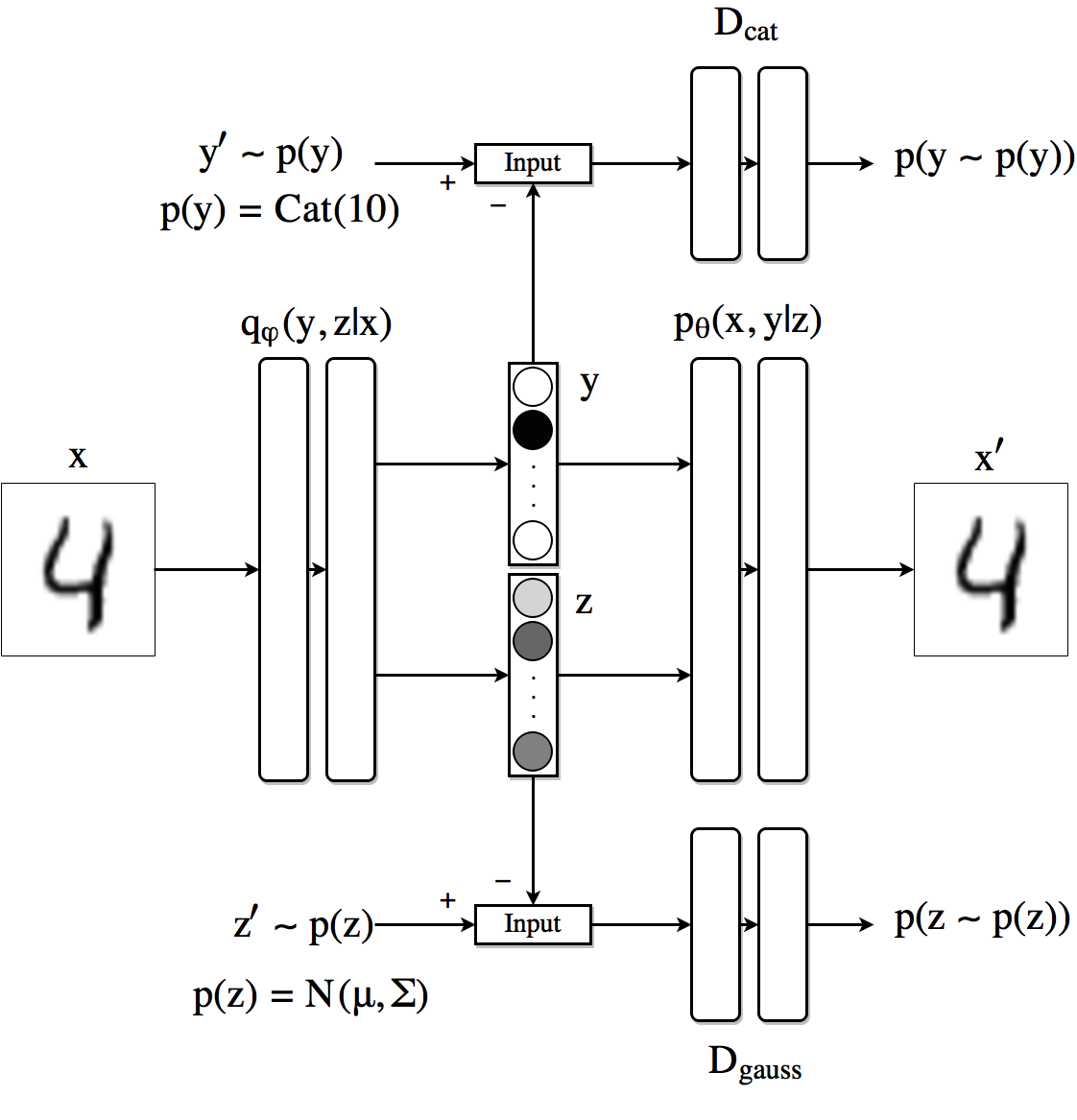
Adversarial autoencoders avoid using the KL divergence altogether by using adversarial learning. In this architecture, a new network is trained to discriminatively predict whether a sample comes from the hidden code of the autoencoder or from the prior distribution
The image shows schematically how AAEs work when we use a Gaussian prior for the latent code (although the approach is generic and can use any distribution). The top row is equivalent to an VAE. First a sample 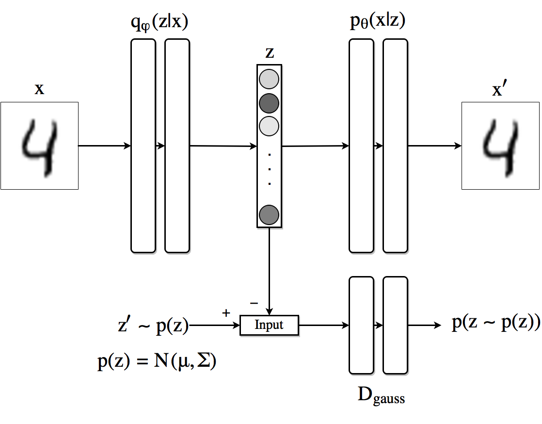 On the adversarial regularization part the discriminator recieves
We can now use the loss incurred by the the generator of the adversarial network (which is the encoder of the autoencoder) instead of a KL divergence for it to learn how to produce samples according to the distribution
The loss of the discriminator is
where
For the adversarial generator we have
Before getting into the training procedure used for this model, we look at how to implement what we have up to now in Pytorch. For the encoder, decoder and discriminator networks we will use simple feed forward neural networks with three 1000 hidden state layers with ReLU nonlinear functions and dropout with probability 0.2.
#Encoder
class Q_net(nn.Module):
    def __init__(self):
        super(Q_net, self).__init__()
        self.lin1 = nn.Linear(X_dim, N)
        self.lin2 = nn.Linear(N, N)
        self.lin3gauss = nn.Linear(N, z_dim)
    def forward(self, x):
        x = F.droppout(self.lin1(x), p=0.25, training=self.training)
        x = F.relu(x)
        x = F.droppout(self.lin2(x), p=0.25, training=self.training)
        x = F.relu(x)
        xgauss = self.lin3gauss(x)
        return xgauss
# Decoder
class P_net(nn.Module):
def __init__(self):
super(P_net, self).__init__()
self.lin1 = nn.Linear(z_dim, N)
self.lin2 = nn.Linear(N, N)
self.lin3 = nn.Linear(N, X_dim)
def forward(self, x):
x = self.lin1(x)
x = F.dropout(x, p=0.25, training=self.training)
x = F.relu(x)
x = self.lin2(x)
x = F.dropout(x, p=0.25, training=self.training)
x = self.lin3(x)
return F.sigmoid(x)# Discriminator
class D_net_gauss(nn.Module):
def __init__(self):
super(D_net_gauss, self).__init__()
self.lin1 = nn.Linear(z_dim, N)
self.lin2 = nn.Linear(N, N)
self.lin3 = nn.Linear(N, 1)
def forward(self, x):
x = F.dropout(self.lin1(x), p=0.2, training=self.training)
x = F.relu(x)
x = F.dropout(self.lin2(x), p=0.2, training=self.training)
x = F.relu(x)
return F.sigmoid(self.lin3(x))Some things to note from this definitions. Frist, since the output of the encoder has to follow a Gaussian distribution, we do not use any nonlinearities at its last layer. The output of the decoder has a sigmoid nonlinearity, this is because we are using the inputs normalized in a way in which their values are within
Once the networks classes are defined, we create an instance of each one and define the optipmizers to be used. In order to have independence in the optimization procedure for the encoder (which is as well the generator of the adversarial network) we define two optimizers for this part of the network as follows:
    torch.manual_seed(10)
    Q, P = Q_net() = Q_net(), P_net(0)     # Encoder/Decoder
    D_gauss = D_net_gauss()                # Discriminator adversarial
    if torch.cuda.is_available():
        Q = Q.cuda()
        P = P.cuda()
        D_cat = D_gauss.cuda()
        D_gauss = D_net_gauss().cuda()
    # Set learning rates
    gen_lr, reg_lr = 0.0006, 0.0008
    # Set optimizators
    P_decoder = optim.Adam(P.parameters(), lr=gen_lr)
    Q_encoder = optim.Adam(Q.parameters(), lr=gen_lr)
    Q_generator = optim.Adam(Q.parameters(), lr=reg_lr)
D_gauss_solver = optim.Adam(D_gauss.parameters(), lr=reg_lr)The training procedure for this architecture for each minibatch is performed as follows:
- Do a forward path through the encoder/decoder part, compute and update the parameteres of the encoder Q and decoder P networks.
    z_sample = Q(X)
    X_sample = P(z_sample)
    recon_loss = F.binary_cross_entropy(X_sample + TINY, X.resize(train_batch_size, X_dim) + TINY)
    recon_loss.backward()
    P_decoder.step()
Q_encoder.step()- Create a latent representation z = Q(x) and a sample z’ from the prior p(z), run each one through the discriminator and compute the score assigned to each (D(z) and D(z’)).
    Q.eval()
    z_real_gauss = Variable(torch.randn(train_batch_size, z_dim) * 5)   # Sample from N(0,5)
    if torch.cuda.is_available():
        z_real_gauss = z_real_gauss.cuda()
    z_fake_gauss = Q(X)
    # Compute discriminator outputs and loss
    D_real_gauss, D_fake_gauss = D_gauss(z_real_gauss), D_gauss(z_fake_gauss)
    D_loss_gauss = -torch.mean(torch.log(D_real_gauss + TINY) + torch.log(1 - D_fake_gauss + TINY))
    D_loss.backward()       # Backpropagate loss
D_gauss_solver.step() # Apply optimization step[- Compute the loss in the discriminator as and backpropagate it through the discriminator network to update its weights. In code,
    Q.eval()    # Not use dropout in Q in this step
    z_real_gauss = Variable(torch.randn(train_batch_size, z_dim))
    if cuda:
        z_real_gauss = z_real_gauss.cuda()
    z_fake_gauss = Q(X)

    D_real_gauss = D_gauss(z_real_gauss)
    D_fake_gauss = D_gauss(z_fake_gauss)
    D_loss_gauss = -torch.mean(torch.log(D_real_gauss + TINY) + torch.log(1 - D_fake_gauss + TINY))
    D_loss.backward()
D_gauss_solver.step()- Compute the loss of the generator network and update Q network accordingly.
        # Generator
        Q.train()   # Back to use dropout
        z_fake_gauss = Q(X)
        D_fake_gauss = D_gauss(z_fake_gauss)

        G_loss = -torch.mean(torch.log(D_fake_gauss + TINY))
        G_loss.backward()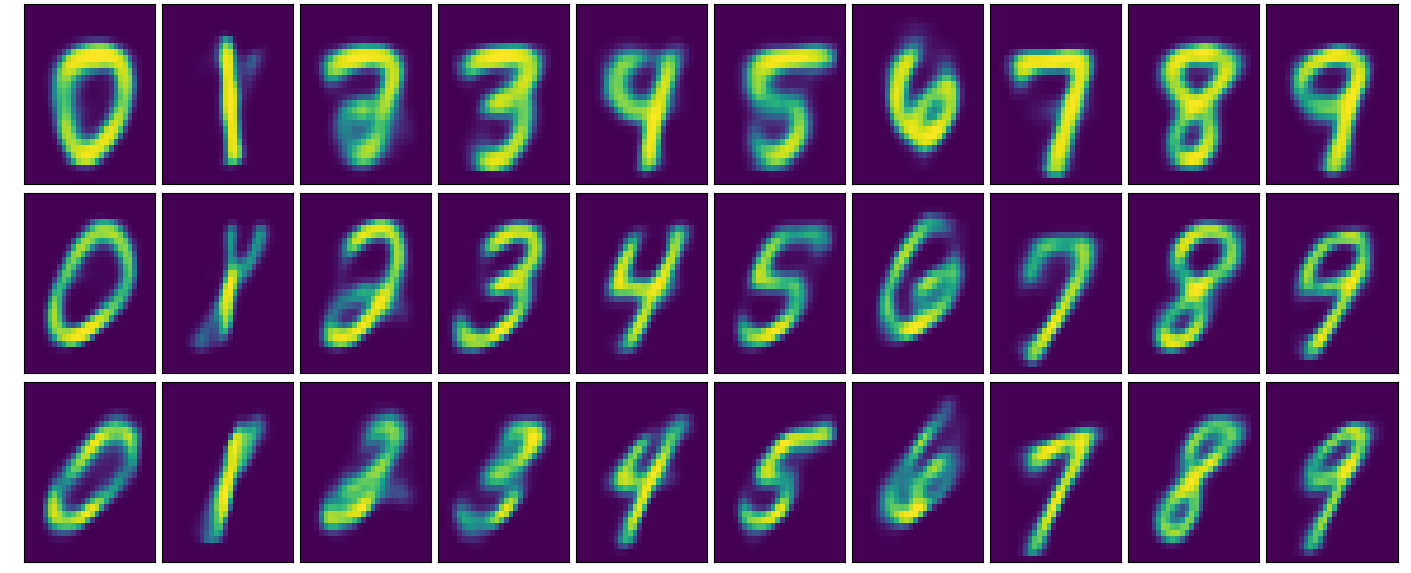
Q_generator.step()Now we attempt to visualize at how the AAE encodes images into a 2-D Gaussian latent representation with standard deviation 5. For this we first train the model and then use the generator part with a code 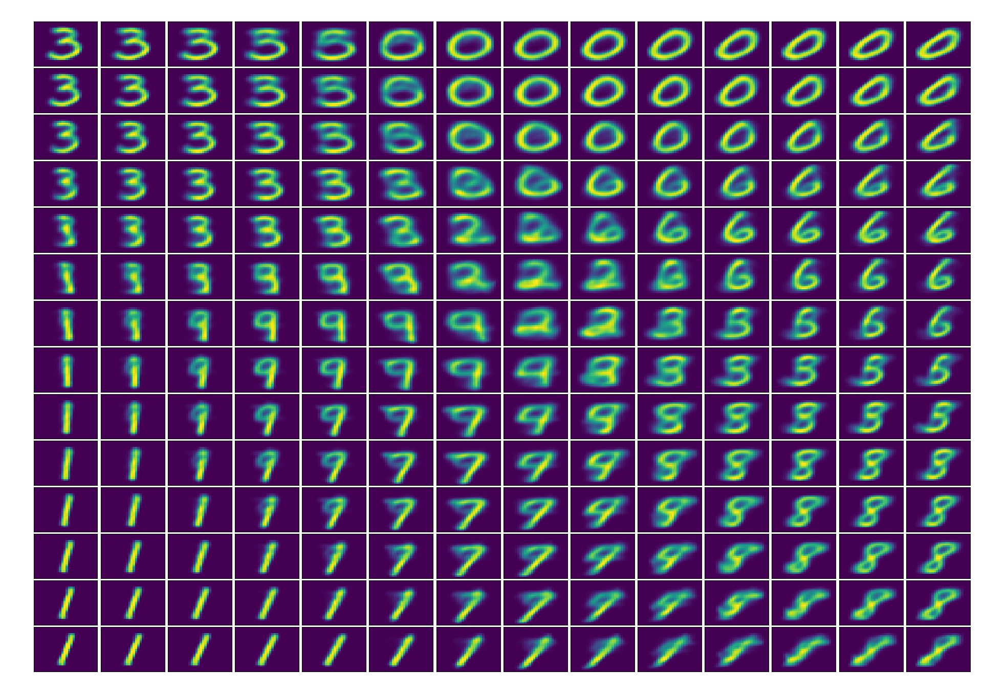
In this step we go one step forward and try to impose certain structure in the latent code
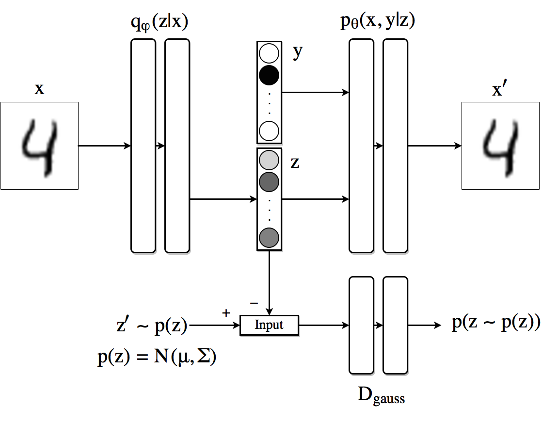
In this setting, the decoder uses the one-hot vector 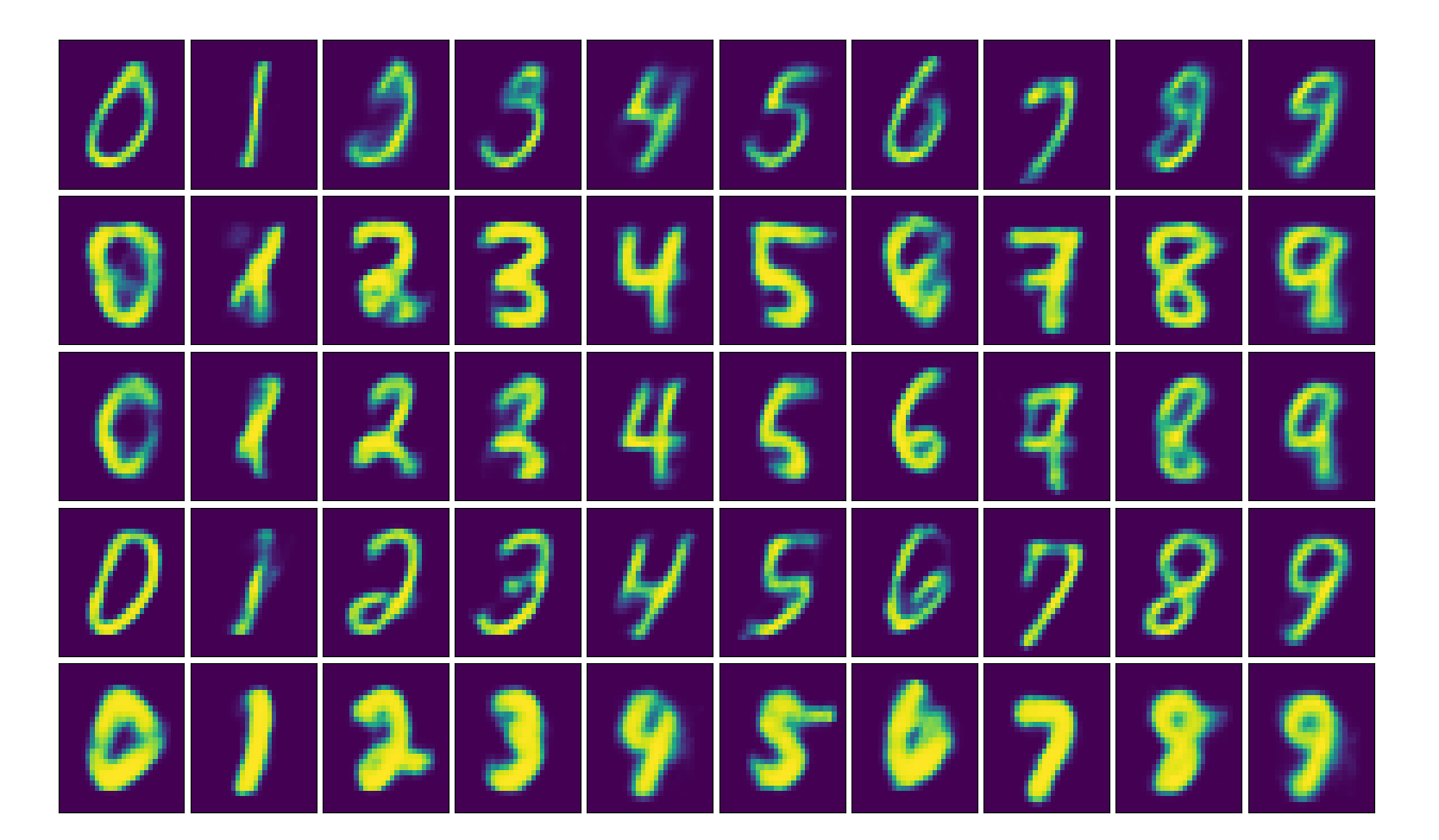
As our last experiment we look an alternative to obtain similar disentanglement results for the case in which we have only few samples of labeled information. We can modify the previous architecture so that the AAE produces a latent code composed by the concatenation of a vector
The unlabeled data contributes to the training procedure by improving the way the enconder creates the hidden code based on the reconstruction loss and improving the generator and discriminator networks for which no labeled information is needed.
It is worth noticing that now, not only we can generate images with fewer labeled information, but also we can classify the images for which we do not have labels by looking at the latent code