In the midst of growing interest in off-policy evaluation (OPE), the research community has produced a number of OPE estimators. One emerging challenge with this trend is that there is a need for practitioners to select and tune appropriate hyper-parameters of OPE estimators for their specific application. However, most OPE papers evaluate the estimator's performance for a single set of arbitrary hyper-parameters and a single arbitrary evaluation policy. Therefore, it is difficult for practitioners to evaluate the estimator's sensitivity to hyper-parameter choices or evaluation policy choices, which is critical in real-world scenarios. Consequently, this type of evaluation procedure fails to answer the following question: which OPE estimator provides an accurate and reliable off-policy evaluation without environment specific hyper-parameter tuning?
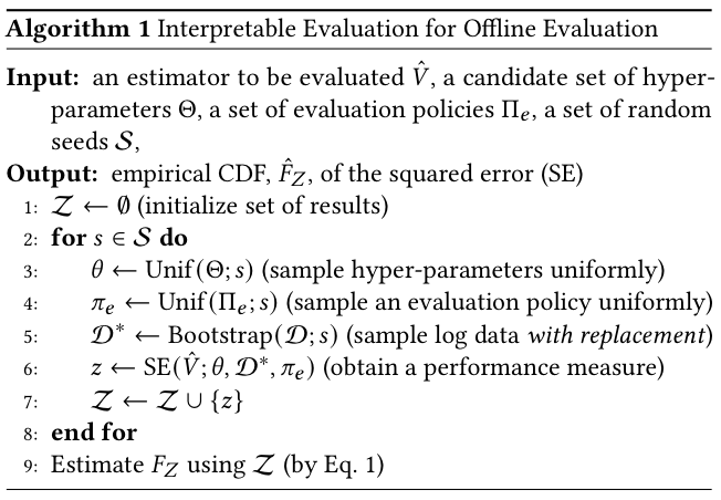
Towards a reliable offline evaluation, we develop a interpretable evaluation procedure for OPE methods that quantifies their sensitivity to hyper-parameter choices and/or evaluation policy choices. Our proposed evaluation procedure is summarized in the figure below:
To evaluate the performance of a single OPE estimator, we prepare a set of candidates for hyper-parameters, evaluation policies, and random seeds, respectively. For each random seed, we (uniformly) randomly choose hyper-parameters and an evaluation policy. Furthermore, we randomly sample log data with replacement via the bootstrap method. Then, we conduct OPE using the specified OPE estimator and obtain a performance measure. We can use the aggregated performance measure to evaluate the performance of the OPE estimator. In particular, we can estimate the cumulative distribution function (CDF) of the performance measure. By repeating this process for each OPE estimator, we can evaluate and compare the performance of the OPE estimators.
You can install pyIEOE using Python's package manager pip.
pip install pyieoeYou can also install pyIEOE from source.
git clone https://github.com/sony/pyIEOE
cd pyIEOE
python setup.py installWe provide a Python package that allows practitioners to easily execute the proposed robust and interpretable evaluation procedure for OPE methods. For example with actual code, please look at ./examples/. (Note: this package is built with the intention of being used along with the Open Bandit Pipeline (obp))
Before we use pyIEOE, we need to prepare logged bandit feedback data and evaluation policies (action distributions and ground truth policy value for each action distribution). This can be done by using the dataset module of obp as follows.
# here we show an example using SyntheticBanditDataset from obp
from obp.dataset import (
    SyntheticBanditDataset,
    logistic_reward_function,
    linear_behavior_policy
)

# initialize SyntheticBanditDataset class
dataset = SyntheticBanditDataset(
    n_actions=10,
    dim_context=5,
    reward_type="binary", # "binary" or "continuous"
    reward_function=logistic_reward_function,
    behavior_policy_function=linear_behavior_policy,
    random_state=12345,
)
# obtain synthetic logged bandit feedback data
n_rounds = 10000
bandit_feedback = dataset.obtain_batch_bandit_feedback(n_rounds=n_rounds)

# prepare action distribution and ground truth policy value for each evaluation policy
action_dist_a = #...
ground_truth_a = #...
action_dist_b = #...
ground_truth_b = #...Then, we define hyperparameter spaces for OPE estimators and regression models. (Note: we can also set this after initializing the InterpretableOPEEvaluator class.)
# hyperparameter space for ope estimators
lambda_ = {
    "lower": 1e-3,
    "upper": 1e2,
    "log": True,
    "type": float
}
K = {
    "lower": 1,
    "upper": 5,
    "log": False,
    "type": int
}
dros_param = {"lambda_": lambda_, "K": K}
sndr_param = {"K": K}

# hyperparameter space for regression model
C = {
    "lower": 1e-3,
    "upper": 1e2,
    "log": True,
    "type": float
}
n_estimators = {
    "lower": 20,
    "upper": 200,
    "log": True,
    "type": int
}
lr_hp = {"C": C}
rf_hp = {"n_estimators": n_estimators}Then, we initialize the InterpretableOPEEvaluator class.
# import InterpretableOPEEvaluator
from pyieoe.evaluator import InterpretableOPEEvaluator

# import other necessary packages
from sklearn.linear_model import LogisticRegression
from sklearn.ensemble import RandomForestClassifier as RandomForest
from obp.ope import (
    DoublyRobustWithShrinkage,
    SelfNormalizedDoublyRobust,
)

# initialize InterpretableOPEEvaluator class
evaluator = InterpretableOPEEvaluator(
    random_states=np.arange(1000),
    bandit_feedbacks=[bandit_feedback],
    evaluation_policies=[
        (ground_truth_a, action_dist_a),
        (ground_truth_b, action_dist_b),
    ],
    ope_estimators=[
        DoublyRobustWithShrinkage(),
        SelfNormalizedDoublyRobust(),
    ],
    regression_models=[
        LogisticRegression,
        RandomForest,
    ],
    regression_model_hyperparams={
        LogisticRegression: lr_hp,
        RandomForest: rf_hp,
    },
    ope_estimator_hyperparams={
        DoublyRobustWithShrinkage.estimator_name: dros_param,
        SelfNormalizedDoublyRobust.estimator_name: sndr_param,
    }
)
We can now perform the interpretable OPE evaluation by calling built in methods.
# estimate policy values
policy_value = evaluator.estimate_policy_value()

# compute squared errors
se = evaluator.calculate_squared_error()
We can visualize the results as well.
# visualize CDF of squared errors for each OPE estimator
evaluator.visualize_cdf(fig_dir="figures", fig_name="cdf.png")
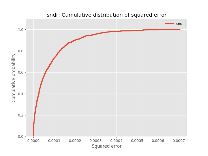
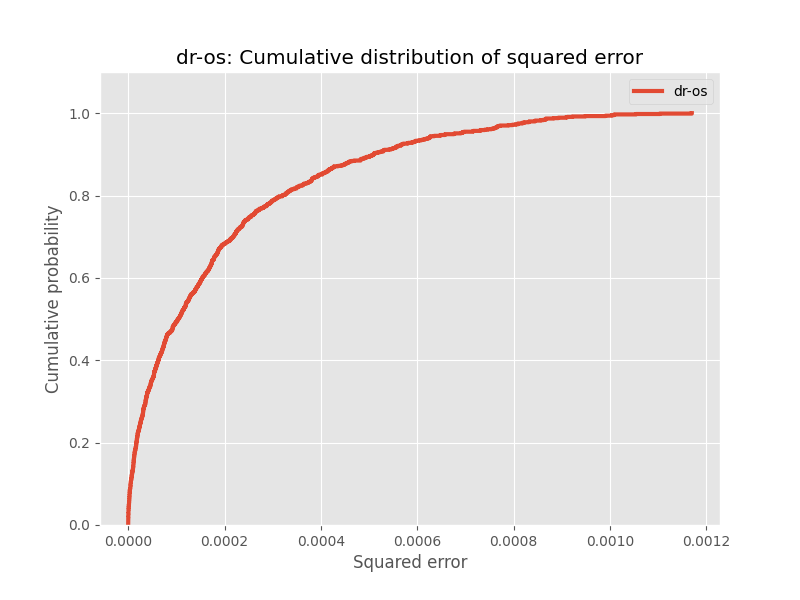
After calling InterpretableOPEEvaluator().visualize_cdf(), we can expect to obtain figures similar to the ones shown below:
In this example, we evaluate and compare Self Normalized Doubly Robust (SNDR) and Doubly Robust with Shrinkage (DRos). Each of these figures visualizes the CDF of the squared error for an OPE estimator. The y-axis represents the cumulative probability, and the x-axis represents the squared error. For instance, if we look at the figure for SNDR, we can tell that with a probability of 80%, the squared error of the SNDR estimator is less than 0.0002. On the other hand, if we look at the figure for DRos, we can tell that with a probability of 80%, the squared error of the DRos estimator is less than 0.0003.
To compare the estimators, we can run the following:
# visualize CDF of squared errors for each OPE estimator
evaluator.visualize_cdf_aggregate(fig_dir="figures", fig_name="cdf.png")
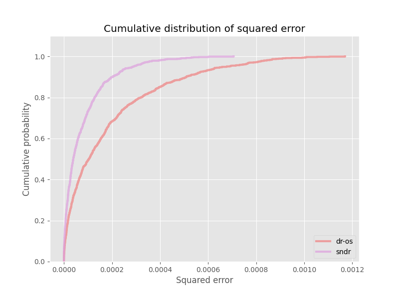
After calling InterpretableOPEEvaluator().visualize_cdf_aggregate(), we can expect to obtain figures similar to the one shown below:
This figure plots the CDFs of all OPE estimators. This allows for an easy comparison between the OPE estimators. In particular, these figures suggests that the SNDR estimator outperforms the DRos estimator.
If you use our package in your work, please cite our paper:
Bibtex:
@inproceedings{saito2021evaluating,
  title={Evaluating the Robustness of Off-Policy Evaluation},
  author={Saito, Yuta and Udagawa, Takuma and Kiyohara, Haruka and Mogi, Kazuki and Narita, Yusuke and Tateno, Kei},
  booktitle = {Proceedings of the 15th ACM Conference on Recommender Systems},
  pages={xxx},
  year={2021}
}
- Kazuki Mogi (Stanford University / Hanjuku-kaso Co., Ltd.)
- Haruka Kiyohara (Tokyo Institute of Technology / Hanjuku-kaso Co., Ltd.)
- Yuta Saito (Cornell University / Hanjuku-kaso Co., Ltd.)
- Yuta Saito (Cornell University / Hanjuku-kaso Co., Ltd.)
- Takuma Udagawa (Sony Group Corporation)
- Haruka Kiyohara (Tokyo Institute of Technology / Hanjuku-kaso Co., Ltd.)
- Kazuki Mogi (Stanford University / Hanjuku-kaso Co., Ltd.)
- Yusuke Narita (Hanjuku-kaso Co., Ltd. / Yale University)
- Kei Tateno (Sony Group Corporation)
For any question about the paper and package, feel free to contact: saito@hanjuku-kaso.com
This software is released under the MIT License, see LICENSE for the detail.


