 |
hyperdrive: an algorithmic trading library |
|---|
hyperdrive is an algorithmic trading library that powers quant research firm ![]() FORCEPU.SH.
FORCEPU.SH.
Unlike other backtesting libraries, hyperdrive specializes in data collection and quantitative research.
In the examples below, we explore how to:
- store market data
- create trading strategies
- test strategies against historical data (backtesting)
- execute orders.
You will need Python 3.8+
To install the necessary packages, run
pythom -m pip install hyperdrive -U
Most secrets must be passed as environment variables. Future updates will allow secrets to be passed directly into class object (see example on order execution).
Pre-requisites:
- a Polygon API key
- an AWS account and an S3 bucket
Environment Variables:
POLYGONAWS_ACCESS_KEY_IDAWS_SECRET_ACCESS_KEYAWS_DEFAULT_REGIONS3_BUCKET
from hyperdrive import DataSource
from DataSource import Polygon, MarketData

# Polygon API token loaded as an environment variable (os.environ['POLYGON'])

symbol = 'TSLA'
timeframe = '7d'

md = MarketData()
poly = Polygon()

poly.save_ohlc(symbol=symbol, timeframe=timeframe)
df = md.get_ohlc(symbol=symbol, timeframe=timeframe)

print(df)
Output:
           Time     Open       High      Low    Close       Vol
2863 2021-11-10  1010.41  1078.1000   987.31  1067.95  42802722
2864 2021-11-11  1102.77  1104.9700  1054.68  1063.51  22396568
2865 2021-11-12  1047.50  1054.5000  1019.20  1033.42  25573148
2866 2021-11-15  1017.63  1031.9800   978.60  1013.39  34775649
2867 2021-11-16  1003.31  1057.1999  1002.18  1054.73  26542359
Much of this code is still closed-source, but you can take a look at the Historian class in the History module for some ideas.
We use vectorbt to backtest strategies.
from hyperdrive import History, DataSource, Constants as C
from History import Historian
from DataSource import MarketData

hist = Historian()
md = MarketData()

symbol = 'TSLA'
timeframe = '1y'

df = md.get_ohlc(symbol=symbol, timeframe=timeframe)

holding = hist.buy_and_hold(df[C.CLOSE])
signals = hist.get_optimal_signals(df[C.CLOSE])
my_strat = hist.create_portfolio(df[C.CLOSE], signals)

metrics = [
    'Total Return [%]', 'Benchmark Return [%]',
    'Max Drawdown [%]', 'Max Drawdown Duration',
    'Total Trades', 'Win Rate [%]', 'Avg Winning Trade [%]',
    'Avg Losing Trade [%]', 'Profit Factor',
    'Expectancy', 'Sharpe Ratio', 'Calmar Ratio',
    'Omega Ratio', 'Sortino Ratio'
]

holding_stats = holding.stats()[metrics]
my_strat_stats = my_strat.stats()[metrics]

print(f'Buy and Hold Strat\n{"-"*42}')
print(holding_stats)

print(f'My Strategy\n{"-"*42}')
print(my_strat_stats)

# holding.plot()
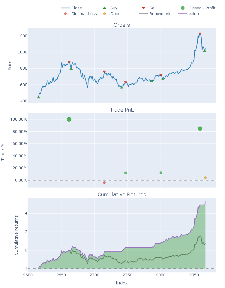
my_strat.plot()
Output:
Buy and Hold Strat
------------------------------------------
Total Return [%]                138.837436
Benchmark Return [%]            138.837436
Max Drawdown [%]                 36.246589
Max Drawdown Duration    186 days 00:00:00
Total Trades                             1
Win Rate [%]                           NaN
Avg Winning Trade [%]                  NaN
Avg Losing Trade [%]                   NaN
Profit Factor                          NaN
Expectancy                             NaN
Sharpe Ratio                      2.206485
Calmar Ratio                      6.977133
Omega Ratio                       1.381816
Sortino Ratio                     3.623509
Name: Close, dtype: object

My Strategy
------------------------------------------
Total Return [%]                364.275727
Benchmark Return [%]            138.837436
Max Drawdown [%]                  35.49422
Max Drawdown Duration    122 days 00:00:00
Total Trades                             6
Win Rate [%]                          80.0
Avg Winning Trade [%]            52.235227
Avg Losing Trade [%]             -3.933059
Profit Factor                     45.00258
Expectancy                      692.157004
Sharpe Ratio                      4.078172
Calmar Ratio                     23.220732
Omega Ratio                       2.098986
Sortino Ratio                     7.727806
Name: Close, dtype: object
Pre-requisites:
- a Binance.US API key
Environment Variables:
BINANCE
from pprint import pprint
from hyperdrive import Exchange
from Exchange import Binance

# Binance API token loaded as an environment variable (os.environ['BINANCE'])

bn = Binance()

# use 45% of your USD account balance to buy BTC
order = bn.order('BTC', 'USD', 'BUY', 0.45)

pprint(order)
Output:
{'clientOrderId': '3cfyrJOSXqq6Zl1RJdeRRC',
 'cummulativeQuoteQty': 46.8315,
 'executedQty': 0.000757,
 'fills': [{'commission': '0.0500',
            'commissionAsset': 'USD',
            'price': '61864.6400',
            'qty': '0.00075700',
            'tradeId': 25803914}],
 'orderId': 714855908,
 'orderListId': -1,
 'origQty': 0.000757,
 'price': 0.0,
 'side': 'SELL',
 'status': 'FILLED',
 'symbol': 'BTCUSD',
 'timeInForce': 'GTC',
 'transactTime': 1637030680121,
 'type': 'MARKET'}
Use the scripts provided in the scripts/ directory as a reference since they are actually used in production daily.
Available data collection functions:


